Cosmetics Spending and Recession Resilience in the United States
Abstract
This paper assesses whether a grouped cosmetics and perfume consumption category holds up better than clothing after US business cycle peaks. A locally locked analysis plan specifies nine NBER peaks from April 1960 to February 2020 and a frozen vintage of BEA monthly quantity indexes spanning January 1959 to August 2026. The primary statistic is the mean cosmetics minus clothing gap twelve months after each peak, relative to each category's preceding endpoint growth trend. The estimated gap is 1.788 log points, with a one-sided calendar-placebo probability of 0.0652, a prespecified Benjamini-Hochberg adjusted value of 0.0652, and positive gaps in four of nine episodes. A rough episode-bootstrap interval is [-1.859, 6.717]. The primary comparison is not established at the registered threshold. Cosmetics have lower pooled quarterly growth sensitivity than clothing, and the jewelry comparison exceeds its placebo benchmark. Excluding the first recession reverses the primary mean. These findings distinguish pooled consumption sensitivity from resilience across recession episodes. Interpretation is limited by nine linked historical events, the quality and breadth of BEA underlying-detail estimates, and an observational placebo design whose exchangeability and inferential calibration are not established.
Keywords: consumer spending; cosmetics; lipstick effect; business cycles; event study; expenditure sensitivity
1 Introduction
The lipstick effect proposes that consumers favor relatively inexpensive beauty purchases when economic conditions deteriorate. Its empirical meaning varies across studies. A category can grow during a downturn, shrink less than another category, gain expenditure share, or respond less strongly to aggregate consumption growth. Each statement concerns a different outcome and comparison. A positive finding for one does not settle the others.
Hill et al. (2012) examine monthly retail spending shares and experiments in which recession cues alter stated product preferences. Their account emphasizes mating motives. MacDonald and Dildar (2020) use Consumer Expenditure Survey microdata from the Great Recession and report increased cosmetics expenditure among women aged 18 to 40, interpreting their evidence as consistent with substitution from clothing. Li et al. (2020) use weekly lipstick scanner data from 2006 to 2016 and report a change in income responsiveness during the Great Recession. These studies differ in population, product definition, nominal or real measurement, and the economic episode being examined. A mechanism involving stated preferences or a subgroup's purchases need not produce the same pattern in aggregate real consumption estimates.
We examine a broad BEA product group over nine business cycle peaks. The outcome includes cosmetics, perfumes, bath and nail preparations, and implements. Clothing and footwear is the main comparison; jewelry and watches provides a second comparison commonly associated with more expensive discretionary purchases. The analysis does not classify individual products by price or prestige. References to small luxuries therefore describe the motivating hypothesis rather than an observed classification of every transaction.
The principal question is whether the grouped beauty category outperforms clothing one year after an economic peak, relative to each category's preceding growth path. Two related questions concern its pooled sensitivity to aggregate spending growth and its performance relative to jewelry. We retain the hypotheses, horizons, trend definition, random seed, and multiple-testing family established in the project's locked analysis plan. All prespecified sensitivity analyses are reported separately from the primary result.
The primary estimate is positive but does not cross the registered threshold. It also conceals substantial variation: cosmetics outperform clothing in four episodes and underperform in five. The first event has an unusually large positive gap and an unusually short available trend window. Lower pooled quarterly sensitivity and a favorable jewelry benchmark coexist with this inconclusive primary result. The paper treats these findings as evidence about distinct historical comparisons, with explicit limits on causal and product-specific interpretation.
2 Data and frozen vintage
The monthly dataset contains 812 observations from January 1959 through August 2026. We use BEA NIPA underlying-detail tables 2.4.3U, 2.4.4U, and 2.4.5U for quantity indexes, price indexes, and nominal personal consumption expenditures respectively. The API identifiers are U20403, U20404, and U20405. Quantity and price indexes use 2017 = 100 and are seasonally adjusted. Nominal values are millions of US dollars at seasonally adjusted annual rates. Table 1 records the selected product identities.
| Category | Line | Quantity | Price | Nominal |
|---|---|---|---|---|
| Cosmetics and perfume group | 139 | DCOSRA | DCOSRG | DCOSRC |
| Clothing and footwear | 104 | DCLORA | DCLORG | DCLORC |
| Jewelry and watches | 63 | DJRYRA | DJRYRG | DJRYRC |
| Total PCE | 1 | DPCERA | DPCERG | DPCERC |
| Goods | 2 | DGDSRA | DGDSRG | DGDSRC |
Notes: Quantity and price indexes have 2017 = 100; monthly values are seasonally adjusted. Nominal values are millions of dollars at annual rates. Table identifiers are U20403, U20404, and U20405.
The main outcome is the official line "Cosmetic / perfumes / bath / nail preparations and implements." The jewelry line is "Jewelry and watches (part of 119)." These two labels differ from the literal labels in the task's analysis specification. The acquisition log documents exact aliases for these verified categories before confirmatory computation. Other line descriptions match directly. Original line labels, numbers, series codes, units, and source notes are preserved in the archive.
BEA underlying-detail values are estimated national accounts aggregates. They should not be described as directly observed retail transactions. BEA (2024, chapter 5, p. 5-7) warns that these detailed estimates are less reliable than higher-level published categories and may rely more on judgmental trends or less reliable source data. The broad historical coverage is valuable, but the measurement system can obscure product-level behavior and can change with revisions.
The NBER chronology supplies the nine peak and trough pairs in Table 2. A peak is the final expansion month; the subsequent month begins the recession, and the trough month is included in the recession. FRED's USREC indicator supplies monthly shading and descriptive recession averages (NBER, n.d.; Federal Reserve Bank of St. Louis, n.d.). Event time is anchored on the peak. A twelve-month endpoint may lie in a contraction or in a recovery; the statistic measures performance after peaks, not exclusively during months classified as recession.
| Peak | Trough |
|---|---|
| 1960-04 | 1961-02 |
| 1969-12 | 1970-11 |
| 1973-11 | 1975-03 |
| 1980-01 | 1980-07 |
| 1981-07 | 1982-11 |
| 1990-07 | 1991-03 |
| 2001-03 | 2001-11 |
| 2007-12 | 2009-06 |
| 2020-02 | 2020-04 |
Notes: Peak months are the final expansion months; recession shading begins the following month and includes the trough. The twelve-month statistic can include recovery months.
Additional FRED inputs are the cosmetics CPI series CUUR0000SEGB02, apparel CPI series CPIAPPSL, and unemployment rate UNRATE. Cosmetics CPI is not seasonally adjusted; apparel CPI and unemployment are seasonally adjusted. Both CPI series use 1982-1984 = 100. The unemployment rate is the CPS U-3 percentage (BLS, 2025, 2026). These variables support descriptive price comparisons and the registered intensity regression rather than the primary quantity-index event study.
The frozen API files have UTC pull-date filenames of October 2, 2026. Their acquisition and initial verification occurred on October 1 in New York time. BEA source notes identify September 30, 2026 as the table revision date. Full production times, FRED update metadata, sanitized requests, and checksums are archived. The paper uses this fixed historical vintage rather than the latest values now returned by live source pages.
All fifteen selected BEA series are complete, finite, and positive over the dataset span. There are no gaps in the monthly index. No missing values were filled. Cosmetics CPI begins in December 1977; its earlier months remain missing. October 2025 is missing in both CPI inputs and UNRATE. That omission affects descriptive comparisons and the intensity regression, while the quantity-index tests retain complete inputs.
3 Analysis plan and methods
3.1 Local analysis lock
The machine-readable specification was locked on October 1, 2026 and committed before confirmatory statistics were computed. The original plan commit is 647aa46062826879af1cb9afdc0f013ce49c1784. Acquisition compatibility was logged in da9a8bd726d1079092350c23c5d54496ac4071ea before confirmation; this latter hash appears in the archived results. The config remains byte-identical to its original locked version. This is a locally committed analysis plan, not an externally registered or independently timestamped protocol.
3.2 Event paths and hypotheses
Let Q denote a monthly quantity index, c a product category, t0 a peak month, and h the number of months from the peak. Let t_min denote the first available data month and p index the nine registered peak episodes. For charts, we index each category to 100 at its peak value and show h from -12 through +24.
The expected growth path is defined by the log change between the peak and the observation 36 months earlier. When the data begin later than that earlier endpoint, the first available month is used and the denominator is the actual elapsed number of months.
This is an endpoint growth rate rather than a regression trend fitted through every prior observation. The April 1960 peak has only fifteen months of prior data, beginning January 1959. Its denominator is fifteen. The abnormal path subtracts the continuation of that endpoint growth rate from the observed log change.
A is measured in log points. Positive values indicate growth above the category's preceding path; negative values indicate a shortfall. The cosmetics minus clothing gap and its primary average at twelve months are defined as follows.
H1 asks whether this mean indicates an unusually favorable cosmetics comparison after real peaks. H1c applies the same definitions with jewelry replacing clothing. Their registered direction is greater. The analysis evaluates a calendar-placebo benchmark; it does not use a conventional one-sample test that assumes independent recession gaps with population mean zero.
3.3 Calendar placebo and supplementary uncertainty
An eligible fake peak must have a full 36-month trend window, at least 24 future months, and distance of at least 24 months from every registered real peak. There are 402 eligible months. We compute each candidate's gap once, then draw 5,000 subsets of nine distinct candidates. Sampling is without replacement within a subset; the same subset may reappear across draws. The random generator is numpy.random.default_rng with seed 42. The upper-tail probability uses the plus-one convention below, where B is the draw count and T_b is a fake-date mean.
The code enumerates all distinct subsets if their number does not exceed the configured draw count; that branch is not used for the main sample. The plus-one convention prevents a zero Monte Carlo estimate under the specified reference procedure (Phipson and Smyth, 2010). It does not make recession dates exchangeable with fake dates or provide randomized causal identification.
We also report a binomial sign summary and a percentile bootstrap with 10,000 resamples of the observed recession gaps. The latter resamples from the observed empirical distribution, following the bootstrap approach introduced by Efron (1979). The sign summary counts positive gaps, using a reference success probability of one half. The bootstrap interval is labelled rough because nine economically linked historical episodes provide little information about its coverage. Neither summary adds a primary hypothesis to the multiple-testing family. The placebo probability describes timing relative to the candidate calendar; the bootstrap describes variation when the nine actual episodes are resampled. Their reference distributions differ.
3.4 Quarterly growth sensitivity
H1b asks whether cosmetics growth is less sensitive to aggregate consumption growth than clothing growth. Each quarterly level is the arithmetic mean of its three monthly quantity indexes. Only complete quarters are used. Growth is 100 times the first difference of log quarterly levels.
We regress the cosmetics minus clothing growth difference on total PCE growth, with an intercept. The null comparison is a zero slope difference; the registered alternative is negative. We also estimate each category's own slope against total growth for descriptive comparison.
There are 269 quarterly growth observations from 1959Q2 through 2026Q2. The incomplete 2026Q3 is excluded. Standard errors use Newey-West HAC covariance with four quarterly lags (Newey and West, 1987). The software uses an asymptotic normal reference for the coefficient-to-standard-error ratio. The slopes measure historical growth associations. Total consumption includes the category outcomes, so it is not an external source of exogenous variation.
3.5 Multiple testing and registered sensitivity analyses
We apply the prespecified Benjamini-Hochberg adjustment across H1, H1b, and H1c, using a nominal threshold of 0.05 (Benjamini and Hochberg, 1995). Raw and adjusted values are reported. The original BH result assumes independent test statistics; broader validity requires calibrated probabilities and suitable dependence conditions. These tests share products, dates, and observations. We have not established the exchangeability or dependence assumptions needed for an unconditional five-percent false-discovery guarantee.
The event sensitivities drop the 2020, July 1981, or 1960 peak; change the horizon to 6, 18, or 24 months; change the trend window to 24 or 48 months; set trend growth to zero; replace clothing with goods; and split peaks before versus from 2000. Fake anchors continue to exclude all registered real peaks and retain at least 24 future months, with the full variant trend window. The period splits use the same all-era candidate pool, so they are descriptive comparisons rather than a formal structural-break test. Significant unadjusted sensitivity probabilities are not promoted over H1.
The final registered sensitivity regresses the monthly change in the nominal cosmetics share, in percentage points, on the monthly unemployment-rate change. It includes an intercept and twelve HAC lags, with a two-sided probability because no direction was registered for that row.
4 Results
4.1 Primary clothing comparison
The mean twelve-month cosmetics minus clothing gap is +1.788 log points. The one-sided calendar-placebo probability is 0.06519, and its BH-adjusted value is also 0.06519. The estimate does not pass the registered threshold. The rough bootstrap interval is [-1.859, 6.717], and only four of nine episodes have positive gaps. The supplementary sign probability is 0.74609. Failure to reject the benchmark does not show that the true effect is absent; the estimate is imprecise and heterogeneous.
| Test | Effect | 95% interval | Raw p | BH p | Positive |
|---|---|---|---|---|---|
| H1 | +1.788 | [-1.859, 6.717] rough bootstrap | 0.06519 | 0.06519 | 4/9 |
| H1b | -1.109 | [-1.801, -0.417] HAC | 0.00085 | 0.00254 | - |
| H1c | +5.725 | [-0.538, 12.656] rough bootstrap | 0.01880 | 0.02819 | 6/9 |
Notes: H1 and H1c effects are log points at twelve months; H1b is a quarterly slope difference. Event intervals resample nine episodes and are rough. All tests are one-sided in the registered direction. BH covers only these three comparisons; its validity depends on the stated assumptions.
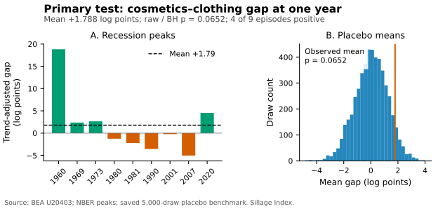
Table 4 gives the gap for every peak. April 1960 contributes +18.828 log points, much larger than the other positive outcomes. The 2007 peak is followed by -5.030, and the 2020 peak by +4.544. A positive average therefore should not be described as a consistent advantage across recessions.
| Peak | Cosmetics minus clothing | Cosmetics minus jewelry |
|---|---|---|
| 1960-04 | +18.828 | +16.756 |
| 1969-12 | +2.375 | +2.643 |
| 1973-11 | +2.647 | -5.287 |
| 1980-01 | -1.258 | +23.595 |
| 1981-07 | -2.236 | -3.230 |
| 1990-07 | -3.552 | +2.110 |
| 2001-03 | -0.228 | +3.766 |
| 2007-12 | -5.030 | +16.585 |
| 2020-02 | +4.544 | -5.408 |
Notes: Effects are 100 times relative log differences after subtracting each category's endpoint growth trend. April 1960 uses a fifteen-month trend. Five clothing comparisons and three jewelry comparisons are negative.
4.2 Quarterly sensitivity and the jewelry comparison
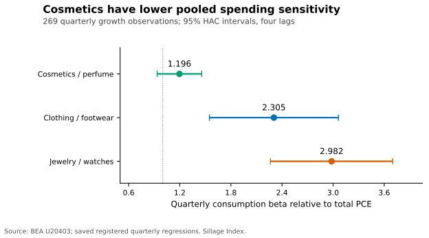
The quarterly slope difference is -1.109, with a HAC interval of [-1.801, -0.417], raw one-sided probability 0.000847, and adjusted value 0.002541. The own-category slopes are 1.196 for cosmetics, 2.305 for clothing, and 2.982 for jewelry. An additional log point of quarterly total consumption growth is associated with a smaller increase in cosmetics growth than in clothing growth. Cosmetics still have a positive association with aggregate growth. These estimates indicate a comparative association under the stated regression model, without demonstrating countercyclical demand or a substitution mechanism.
| Category | Slope | 95% HAC interval |
|---|---|---|
| Clothing | 2.305 | [1.548, 3.062] |
| Cosmetics | 1.196 | [0.935, 1.457] |
| Jewelry | 2.982 | [2.264, 3.700] |
Notes: 269 complete quarterly growth observations, 1959Q2-2026Q2; intercept included; four HAC lags; asymptotic normal inference. Positive slopes indicate procyclical association.
The cosmetics minus jewelry event mean is +5.725 log points, with raw calendar-placebo probability 0.01880 and BH-adjusted value 0.02819. Six of nine episodes are positive. Its rough bootstrap interval, [-0.538, 12.656], includes zero, and its supplementary sign probability is 0.25391. The comparison exceeds the nominal placebo threshold, but uncertainty across the observed episodes remains large. A favorable comparison with expensive discretionary goods is therefore more defensible than a claim of uniform recession resistance.
H1b and H1 answer different questions. The pooled regression uses the full quarterly history, whereas H1 compares nine twelve-month endpoints with category-specific preceding paths. Lower pooled growth sensitivity does not determine the sign of every trend-adjusted event gap. The quarterly regression includes the COVID period; the registered exclusion of the 2020 peak applies to the H1 event statistic only.
4.3 Registered sensitivity analyses
The event mean changes to -0.342 after excluding 1960, with placebo probability 0.62168. Excluding 2020 gives +1.443 with probability 0.13357. For the three peaks from 2000 onward, the mean is -0.238 with probability 0.56509. These results show that the positive full-sample mean depends on the included episodes. Their small samples and shared all-era placebo pool limit claims about changes over time.
| Variant | Mean gap | Placebo p | Positive | Rough 95% interval |
|---|---|---|---|---|
| Exclude 2020 | +1.443 | 0.13357 | 3/8 | [-2.392, 6.908] |
| Exclude July 1981 | +2.291 | 0.03479 | 4/8 | [-1.737, 7.656] |
| Exclude 1960 | -0.342 | 0.62168 | 3/8 | [-2.436, 1.817] |
| Horizon 6 months | +1.561 | 0.01940 | 4/9 | [-1.185, 4.736] |
| Horizon 18 months | +1.000 | 0.25915 | 3/9 | [-2.300, 6.410] |
| Horizon 24 months | +1.032 | 0.30514 | 3/9 | [-3.358, 7.198] |
| Trend 24 months | +1.314 | 0.17157 | 3/9 | [-2.314, 6.329] |
| Trend 48 months | +1.724 | 0.07958 | 5/9 | [-1.989, 6.713] |
| No trend subtraction | +1.477 | 0.07059 | 4/9 | [-2.821, 6.509] |
| Goods comparison | +1.320 | 0.06959 | 5/9 | [-1.608, 5.250] |
| Peaks before 2000 | +2.801 | 0.02519 | 3/6 | [-1.906, 9.659] |
| Peaks from 2000 | -0.238 | 0.56509 | 1/3 | [-5.030, 4.544] |
Notes: These twelve event variants are reported only, use seed 42, 5,000 placebo draws, and 10,000 episode resamples. The intensity regression is the thirteenth variant and is reported in the text. Period subsets use the same all-era placebo pool. Probabilities are unadjusted; no sensitivity replaces H1.
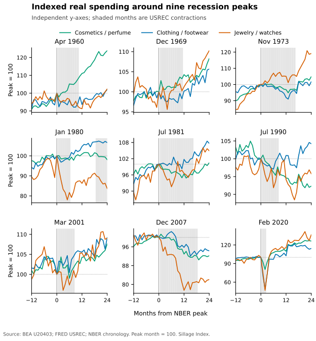
Some sensitivities cross an unadjusted 0.05 threshold, including the six-month horizon and dropping the July 1981 peak. They do not replace the prespecified twelve-month result. The variation across trend windows and horizons is relevant to interpretation even when a particular unadjusted probability is small. Appendix Figure A1 shows the observed paths, including the depth and rebound of the COVID episode.
The intensity estimate is -0.000686981 share percentage points per unemployment percentage point, with HAC interval [-0.001385643, 0.000011681], two-sided probability 0.05396, and 809 complete pairs. The missing October 2025 unemployment level removes both October and November changes. HAC's twelve lags count retained complete observations, so covariance pairs across that gap can span more calendar months. Missing values remain unfilled. This sensitivity does not cross a nominal five-percent threshold and does not identify household substitution.
4.4 Descriptive price and current-reading results
The mean abnormal cosmetics minus total PCE price gap at twelve months is +1.579 log points. The year-over-year BEA cosmetics price change and BLS cosmetics CPI change have correlation 0.9869 over 571 complete pairs from January 1979 through August 2026. This is a correlation of changes rather than trending index levels. BLS prices contribute to BEA estimation, so close agreement is not fully independent validation. The comparison also mixes a seasonally adjusted BEA price index with a nonseasonally adjusted BLS series.
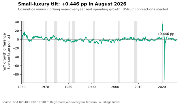
For the accompanying index reading, we compute the difference between arithmetic year-over-year quantity growth in cosmetics and clothing. This descriptive reading differs from the event-study gap, which subtracts a pre-peak log trend.
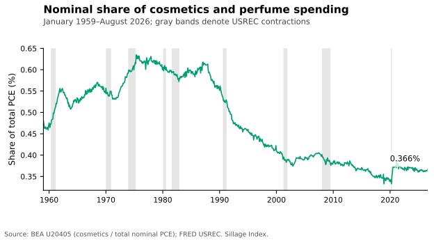
August 2026 has a tilt of +0.446 percentage points, at the 59.25th percentile of its available history. The registered direction rule classifies it as steady: the absolute value of its annual change is less than half the standard deviation of historical annual changes. Its mean during USREC recession months is +1.731 percentage points. This continuous indicator is descriptive and is not added to the three-test family. Appendix Figures A2 and A3 show the nominal share and tilt history.
5 Interpretation and limitations
The primary comparison does not establish a consistent post-peak advantage for the grouped cosmetics category at the registered threshold. The positive mean is accompanied by five negative episode gaps, a wide bootstrap interval, and substantial sensitivity to the first peak. The jewelry comparison and quarterly slope difference concern different benchmarks and provide more favorable evidence within their specified analyses. They should be interpreted alongside the primary uncertainty.
Product aggregation is a central constraint. The outcome combines perfume, cosmetics, bath products, nail products, and implements. It does not separate premium from inexpensive products, fragrance from lipstick, or individual customers from the national aggregate. BEA's warning about underlying-detail quality adds measurement uncertainty. No transaction-level behavior or motive is observed, and group-level evidence cannot determine whether households traded clothing purchases for perfume.
The calendar benchmark has several limitations. Recession timing is observational, and exchangeability between peaks and eligible expansion-period dates has not been established. The candidate rule excludes anchors close to peaks rather than every recession month or every recession-affected trend window. Fake anchors can cluster and their windows can overlap. The full historical pool mixes decades with different product markets and price measurement. Monte Carlo precision does not remove these design assumptions, and the BH adjustment cannot repair invalid input probabilities.
The first peak has a fifteen-month trend whereas every main placebo anchor has thirty-six months. This mismatch is prespecified and transparently retained, but it limits comparability with the placebo anchors. The first event also has an unusually large observed gap. The 1980 and 1981 peaks are eighteen months apart: their twelve-month forward intervals do not directly overlap, while their pre-trend and full event windows overlap and the episodes are economically linked. Resampling nine episodes as though they were independent gives only rough uncertainty summaries.
The pooled regression is an association with aggregate consumption growth, which contains each product category. It uses an asymptotic HAC approximation rather than a randomized instrument. COVID observations remain in that regression, and no registered regression excluding COVID was estimated. The historical comparisons can describe consumption sensitivity but cannot identify a causal income elasticity or the psychological explanations studied in other designs.
The frozen vintage improves reproducibility but leaves revision uncertainty. Later BEA releases may revise the entire history. The paper's archive preserves the exact processed observations and provenance used here, while live quarterly updates can yield different values. The missing unemployment level also changes the spacing of retained observations for one robustness regression. These limitations are concrete reasons to treat the findings as a reproducible historical assessment rather than a general law of luxury consumption.
6 Conclusion
Across nine US business cycle peaks, the registered primary cosmetics minus clothing gap is +1.788 log points with placebo and adjusted values of 0.06519. The grouped cosmetics category has lower pooled quarterly spending sensitivity than clothing, and its jewelry comparison is favorable against the registered calendar benchmark. The event mean reverses after excluding 1960. The evidence supports distinguishing comparative cyclicality from resilience across recession episodes and leaves fragrance-specific substitution mechanisms unresolved.
7 Research transparency
7.1 Data and code availability
The companion reproducibility archive includes the frozen processed monthly dataset, data dictionary and line identities, sanitized source provenance, locked config and analysis plan, saved confirmatory and sensitivity outputs, and the software required to verify the calculations. A separate frozen-paper entrypoint reads those observations directly without network access or credentials. It does not use the production pipeline's moving six-month freshness gate. The dated source files and SHA256 manifest identify the exact vintage; quarterly updates remain a separate operation.
Exact BEA response bodies can echo an API identifier and remain private. The public archive excludes those bodies, all credentials, browser data, and unrelated personal files. Processed public statistical observations and sanitized provenance are sufficient to reproduce the paper's numerical calculations. No synthetic observation or interpolation contributes to the reported results. The numerical pipeline was verified by repeated cached replay and an isolated checkout; the manuscript and archive receive additional checks before release.
7.2 Generative AI assistance and responsibility
OpenAI Codex assisted with code generation, citation discovery, manuscript drafting, and computational review. The reported statistics are computed from the identified official data using the locally locked analysis specification. Independent agent reviews checked the formulas, numerical outputs, source metadata, and chart rendering. These automated reviews do not constitute journal peer review or independent human expert review. The paper is self-published as an AI-assisted working paper and should be evaluated on its data, methods, disclosure, and reproducibility.
7.3 Scope and disclosures
This working paper analyzes aggregate public statistical estimates and contains no individual participant data. It reports no new data collection involving human participants. No institutional endorsement, journal acceptance, or peer-review status is asserted. Funding and competing interests are not declared in this working-paper version. This product uses the FRED API but is not endorsed or certified by the Federal Reserve Bank of St. Louis.
References
- Benjamini, Y., & Hochberg, Y. (1995). Controlling the false discovery rate: A practical and powerful approach to multiple testing. Journal of the Royal Statistical Society: Series B (Methodological), 57(1), 289–300. https://doi.org/10.1111/j.2517-6161.1995.tb02031.x Source
- Efron, B. (1979). Bootstrap methods: Another look at the jackknife. The Annals of Statistics, 7(1), 1–26. https://doi.org/10.1214/aos/1176344552 Source
- Federal Reserve Bank of St. Louis. (n.d.). NBER based Recession Indicators for the United States from the Period following the Peak through the Trough [USREC] [Data set]. FRED. https://fred.stlouisfed.org/series/USREC Source
- Hill, S. E., Rodeheffer, C. D., Griskevicius, V., Durante, K., & White, A. E. (2012). Boosting beauty in an economic decline: Mating, spending, and the lipstick effect. Journal of Personality and Social Psychology, 103(2), 275–291. https://doi.org/10.1037/a0028657 Source
- Li, W., Zhen, C., & Dorfman, J. H. (2020). Modelling with flexibility through the business cycle: Using a panel smooth transition model to test for the lipstick effect. Applied Economics, 52(25), 2694–2704. https://doi.org/10.1080/00036846.2019.1693701 Source
- MacDonald, D., & Dildar, Y. (2020). Social and psychological determinants of consumption: Evidence for the lipstick effect during the Great Recession. Journal of Behavioral and Experimental Economics, 86, 101527. https://doi.org/10.1016/j.socec.2020.101527 Source
- National Bureau of Economic Research. (n.d.). US business cycle expansions and contractions. https://www.nber.org/research/data/us-business-cycle-expansions-and-contractions Source
- Newey, W. K., & West, K. D. (1987). A simple, positive semi-definite, heteroskedasticity and autocorrelation consistent covariance matrix. Econometrica, 55(3), 703–708. https://doi.org/10.2307/1913610 Source
- Phipson, B., & Smyth, G. K. (2010). Permutation p-values should never be zero: Calculating exact p-values when permutations are randomly drawn. Statistical Applications in Genetics and Molecular Biology, 9(1), Article 39. https://doi.org/10.2202/1544-6115.1585 Source
- U.S. Bureau of Economic Analysis. (2024, December). Chapter 5: Personal consumption expenditures. In NIPA Handbook: Concepts and Methods of the U.S. National Income and Product Accounts. https://www.bea.gov/resources/methodologies/nipa-handbook/pdf/chapter-05.pdf Source
- U.S. Bureau of Economic Analysis. (n.d.). Underlying Detail Tables (NIPA) [Data set; tables 2.4.3U, 2.4.4U and 2.4.5U]. https://bea.gov/open-data Source
- U.S. Bureau of Labor Statistics. (2025, April 10). Consumer Price Index: Concepts. Handbook of Methods. https://www.bls.gov/opub/hom/cpi/concepts.htm Source
- U.S. Bureau of Labor Statistics. (2026, May 22). Concepts and definitions (CPS). https://www.bls.gov/cps/definitions.htm Source
Appendix A Descriptive charts
Appendix B Analysis registration and file provenance
The original locally locked analysis specification predates confirmatory computation. Acquisition compatibility affects only the working BEA endpoint, catalog-title validation, and two literal source-label aliases. It does not change the product identities, peak dates, trend definition, twelve-month primary horizon, 5,000 placebo draws, 10,000 bootstrap resamples, or seed 42.
The frozen data comprise 812 monthly observations and twenty variables, with fifteen BEA quantity, price, and nominal series, four FRED inputs, and the computed nominal cosmetics share. All BEA quantity and price indexes are positive. The complete-quarter aggregation produces 269 growth observations. The price-change comparison has 571 complete pairs; intensity has 809 complete monthly changes. The archive's machine-readable file manifest and reproduction report provide the relevant input and output hashes.